Linear Models
Linear models describe the relation between two variables. In a non-technical description we can think about linear model like:
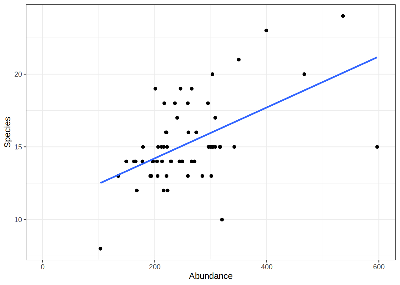
Find a line that is as close as possible to all the points of a scatterplot.
For example, we can use a linear model to depict the relation between the amount of samples animals and the number of different species found in a given area. To create a linear model, we need two vectors (here as two columns of a data.frame) with the matching data pairs (Abundance and Species Number). The lm function then takes a formula with the vector/column names separated by ~. You can interpret the ~ in this case as a function of. So lm(Species ~ Abundance) means: Give me the number of species as a function of species abundance.
library(dplyr)
bd = read.csv("data/crop_species.csv")

bd = bd %>% mutate(Abundance = AraInd + CaraInd + IsoMyrInd,
              Species = AraSpec, CaraSpec, IsoMyrSpec)

lmod = lm(Species ~ Abundance, bd)
lmod
Call:
lm(formula = Species ~ Abundance, data = bd)

Coefficients:
(Intercept)    Abundance
   10.71651      0.01749
Linear Model Summary
Calling the model returns the intercept and slope. To get a more useful output use the summary function. In the following we will go over the output of the summary function on linear models. The explanations are mostly taken from this blog entry: https://feliperego.github.io/blog/2015/10/23/Interpreting-Model-Output-In-R
summary(lmod)
Call:
lm(formula = Species ~ Abundance, data = bd)

Residuals:
    Min      1Q  Median      3Q     Max
-6.3136 -1.2481 -0.2235  1.1245  5.3046

Coefficients:
             Estimate Std. Error t value Pr(>|t|)
(Intercept) 10.716507   0.991039  10.813 1.58e-15 ***
Abundance    0.017491   0.003656   4.784 1.22e-05 ***
---
Signif. codes:  0 '***' 0.001 '**' 0.01 '*' 0.05 '.' 0.1 ' ' 1

Residual standard error: 2.416 on 58 degrees of freedom
Multiple R-squared:  0.2829,    Adjusted R-squared:  0.2706
F-statistic: 22.89 on 1 and 58 DF,  p-value: 1.221e-05
Call
- the function that was used to create the model
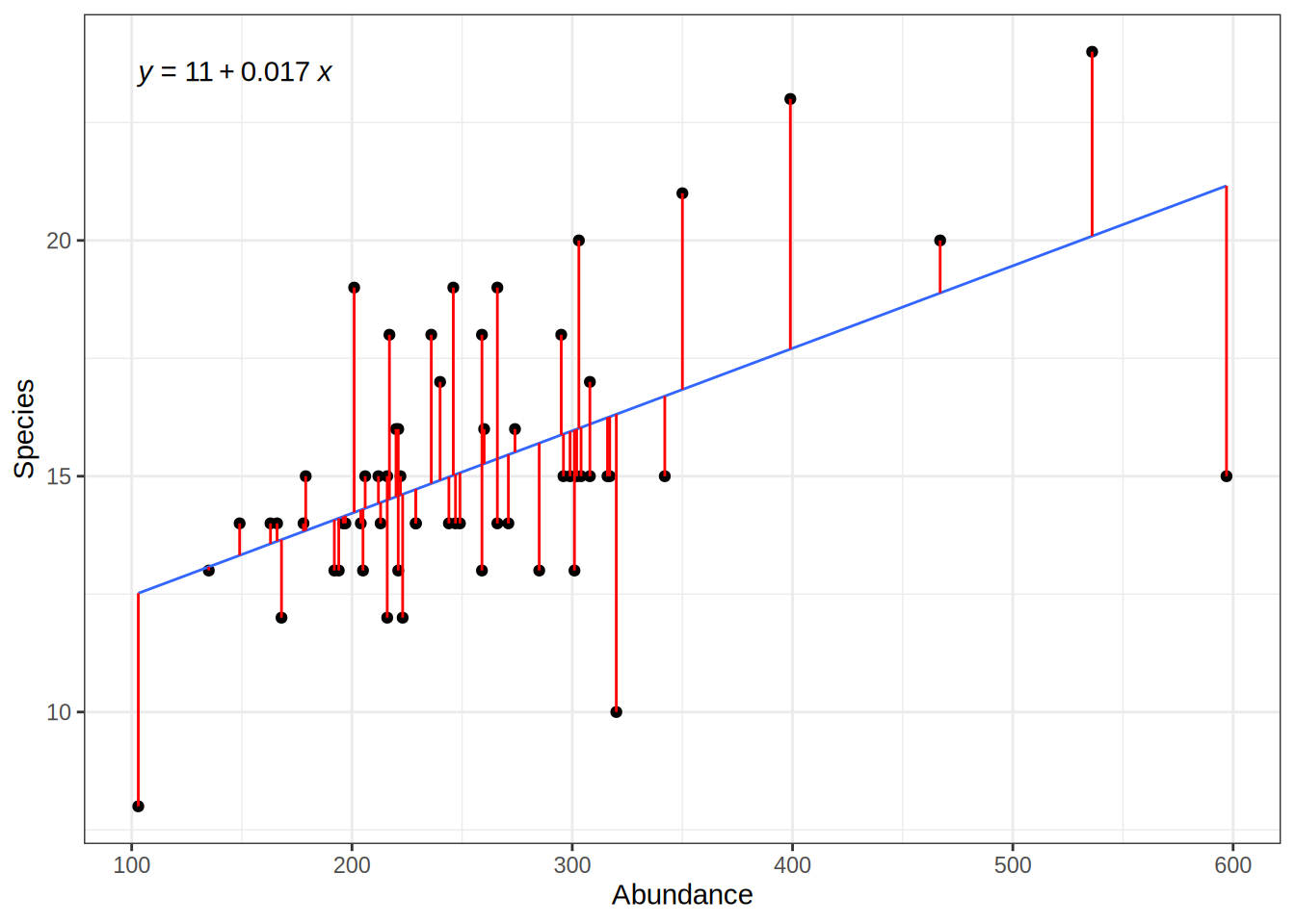
Residuals
- summary statistic of the model error
- “How far away are the real values from the model?”
- should follow a normal distribution (e.g. by plotting a histogram)
hist(lmod$residuals)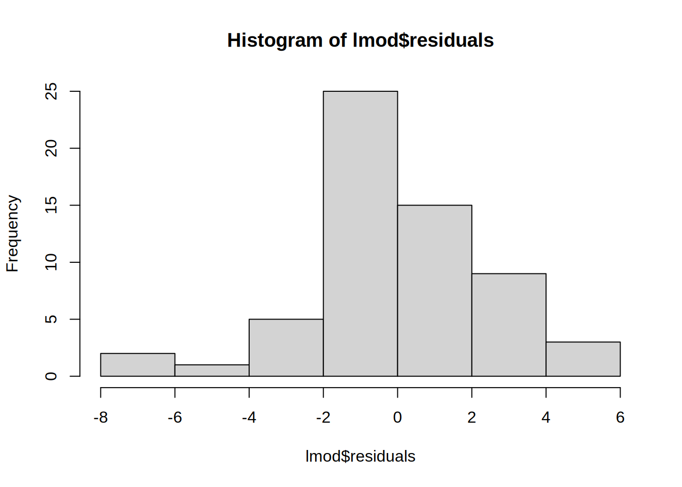
Coefficients
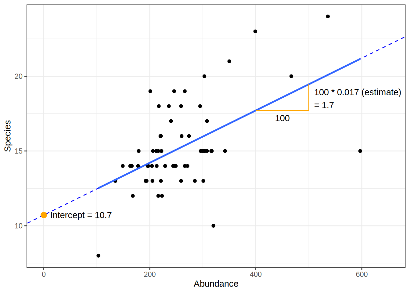
Estimate
- again the slope and intercept
- we can expect to observed at least 10.7 different species on a plot (if we collect 103 animals)
- for each additional animal observed, the species count increases by 0.017
Std. Error
- the expected error of the coefficients
- for each additional animal observed, the species number increases by 0.017 +- 0.0037
t value
- how many standard deviation is the std. error away from zero?
- far away from zero is better. Reduces the probability that the result is due to chance
- usually not interpreted
Pr(>|t|)
- probability that the observed value is larger than t
- small value means that there is a high chance that the relation is not based on chance
- p values < than 0.05 is the convention that we can neglect the H0 hypothesis (the model actually depicts a relation)
Signif. codes
- a legend for the significance level of the p-value
Residuals standard error
- the average deviation of the real values from the model value
- degree of freedom: on how many observations is this value based on?
actual_values = bd$Species
predicted_values = predict(lmod, data.frame(Abundance = bd$Abundance))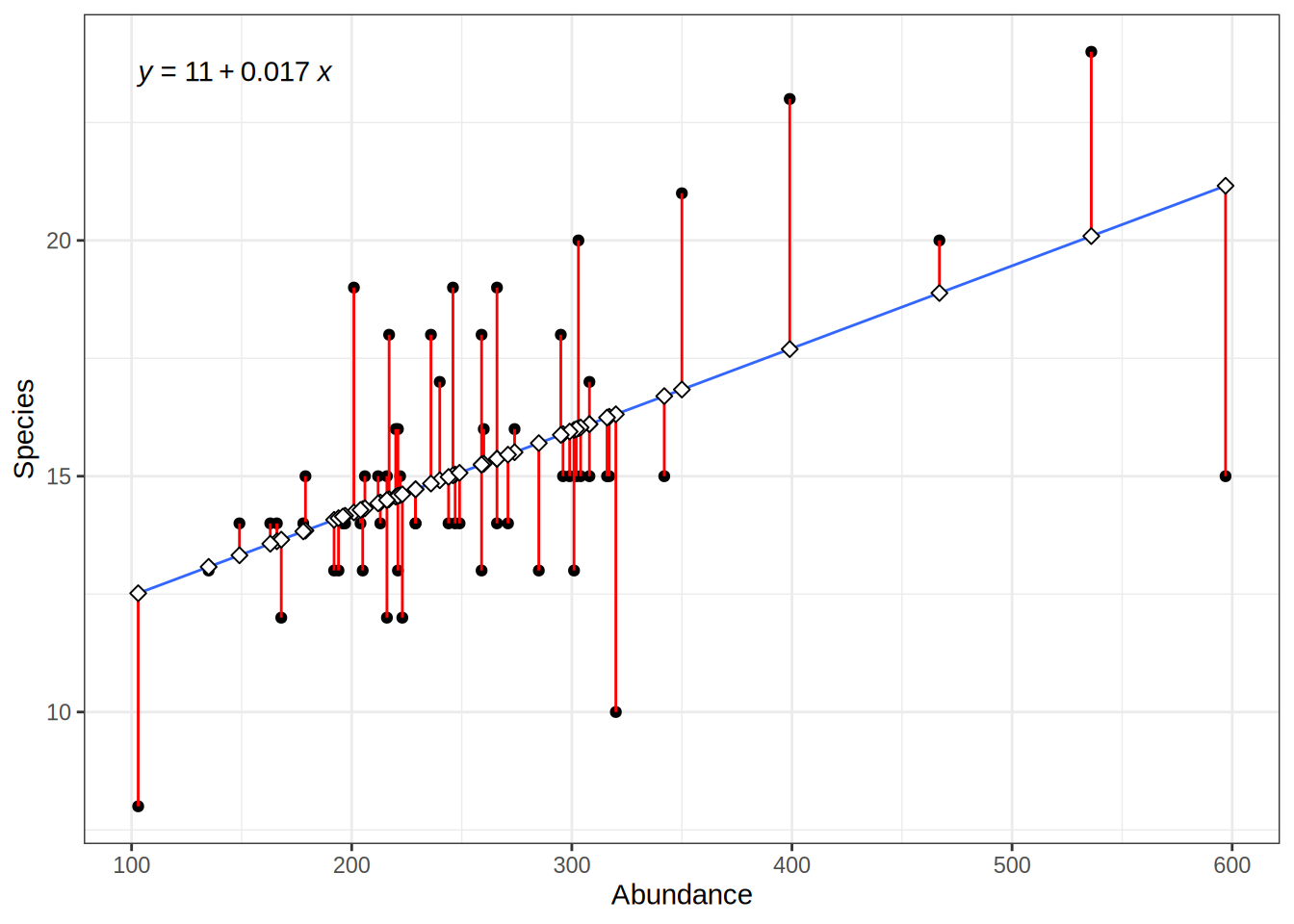
For the specific Abundance values we have in our observed data, we can calculate the error i.e. the deviation of the predicted values from the actual values:
# deviation between actual values and predicted values ("error")
residuals = actual_values - predicted_values

# squared residuals: no negative values, large error values are more severe
squared_error = (actual_values - predicted_values)**2
However, we also want to give estimates of the models error for abundance values that we have not observed.
# number of observations
n = length(actual_values)


# mean squared error
mean(squared_error)
[1] 5.643017# mean squared error with degrees of freedom
sum(squared_error)/(n-1)[1] 5.738662# root mean squared error
sqrt(mean(squared_error))[1] 2.375504# root mean squared error with degrees of freedom == Residuals standard error
sqrt(sum(squared_error)/(n-2))[1] 2.416113Multiple R-squared
- How much of the variance is explained by the model?
- Values between 0 and 1
- 0 means no explanation, 1 means perfect fit
# how much variation is there in the observed values
total_sum_of_squares = sum(((actual_values) - mean(actual_values))**2)


# how much variation is there in the residuals
residual_sum_of_squares = sum((actual_values - predicted_values)**2)


# divide one by the other:
# if both values are similar, this approaches 1
# if residual sum of squares is very low (i.e. the model is good) this value gets smaller
residual_sum_of_squares / total_sum_of_squares
[1] 0.7170542# Rsq: values close to 1 mean, the residual sum of squares error is low compared to the observed variation
1 - residual_sum_of_squares / total_sum_of_squares[1] 0.2829458F-statistics
- Is there a relation between the predictor and the response?
- Is my model better than if all the coefficients are zero?
- Away from 1 is good!
- Depend on number of data points.
Linear Model Plot
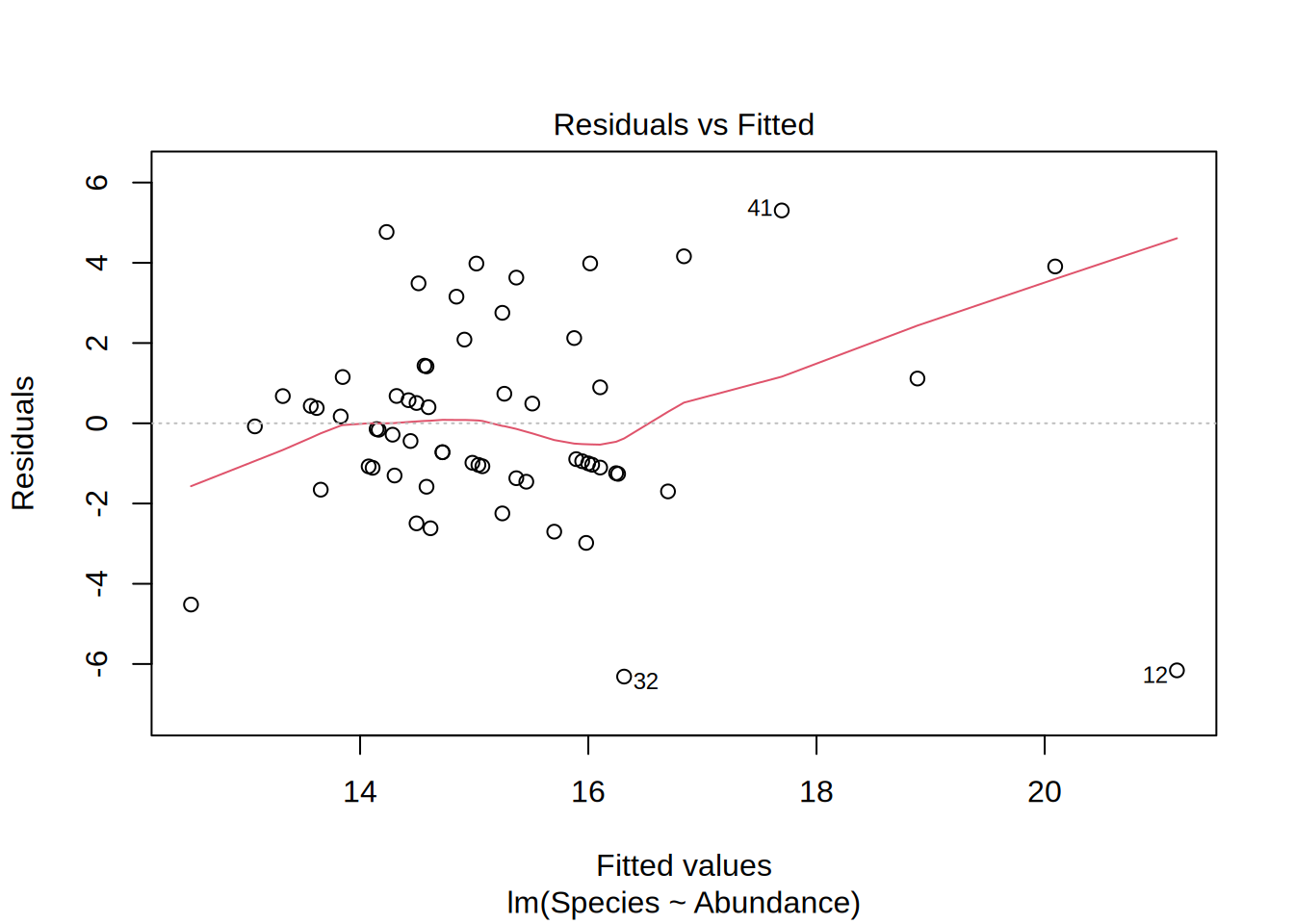
Plotting the linear model gives you 4 different figures that indicate if the model is statistically valid in the first place, i.e. if the residuals follow a normal distribution and if they are homoscedatic.
Residuals vs. Fitted
- Is it actually a linear relation?
- Points randomly scattered around a horizontal line indicates this
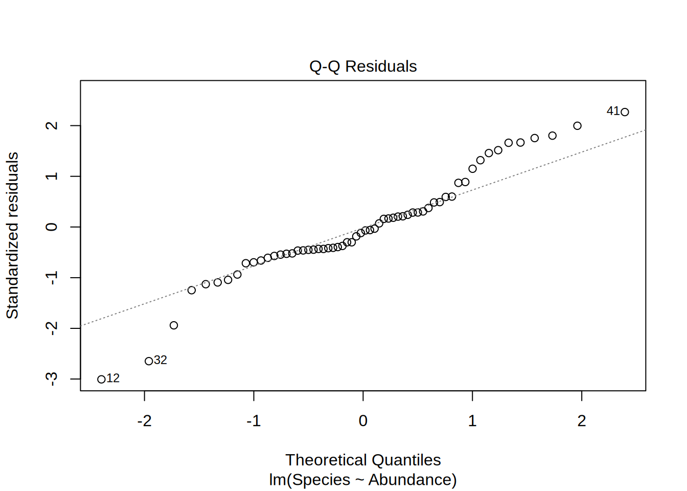
Normal Q-Q
- Are the residuals normally distributed?
- Points on the 1-1 line indicates this
- Depicted are the actual residuals vs. a theoretical normal distribution
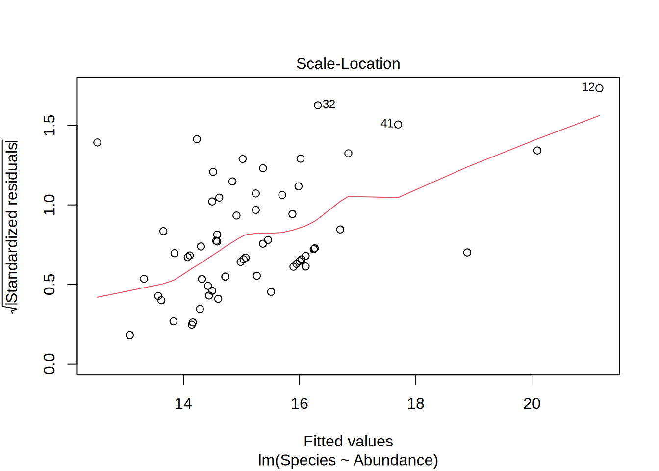
Scale location
- Are the residuals homoscedatic?
- This means that the range of the residuals are more or less equal for the whole data range
- Equally spread points around the line indicates this
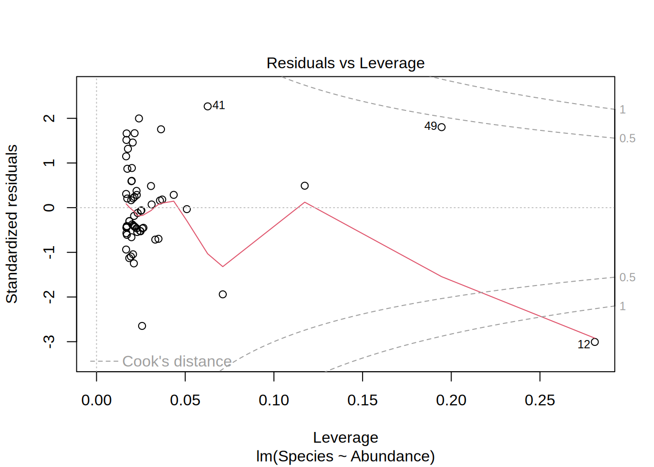
Residuals vs. Levarage
- Are there outliers in the data that have influence on the model?
- In this example, if we would leave out point #12, the model outcome would change.
plot(lmod)